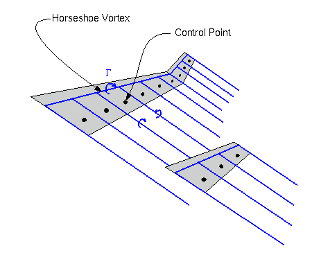
Figure 1: Vortex-lattice method applied to a lifting line
This page describes a non-linear lifting-line method which can predict the lift, drag and pitching moment coefficients of wing and tail configurations at low speeds. The method makes use of experimental section data, and can be used to estimate maximum lift conditions.
Method Description
Limitations
Running the Program
Interpreting the Results
The approach is illustrated in figure 1. Each lifting surface is replaced by a single row of horseshoe vortices, extending along the quarter-chord line. In a traditional vortex-lattice method, a flow-tangency condition is applied at a three-quarter-chord control point aft of each horseshoe vortex, leading to a system of linear equations for the unknown vortex strengths. In the current program, this flow-tangency condition is modified to include the deviation of experimental section data from the theoretical thin-airfoil lift curve. As this deviation depends on the local angle of attack, which in turn depends on the velocity field induced by the horseshoe vortices, the resulting problem is non-linear, and is solved iteratively.

Figure 1: Vortex-lattice method applied to a lifting line
In general the method can predict total forces quite accurately, with
the exception of the
The prediction of maximum lift relies on the choice of experimental data, for which the airfoil section, its roughness and Reynolds number should be as close to the anticipated situation as possible. Spanwise load distributions computed beyond the stall of the first airfoil section will likely be unrealistic, as wing stall includes highly three-dimensional processes which cannot be simulated here. In spite of this, the prediction of CLmax is normally pretty good, and the reasonable agreement of post-stall force coefficients shows that at least some of the features of post-stall stall behaviour can be approximated with the non-linear lifting-line technique.
Two components of drag are predicted, profile drag (CDp on the results page)
and induced drag (CDi on the results page). The profile drag is estimated
using the provided section Cd data, evaluated at the local angle of attack
computed with the vortex-lattice method, and then integrated along the span.
The induced drag is computed via force integration, which is not
always reliable for a line of horseshoe vortices. Although a correction
has been applied, be sure to check the computed induced drag
value with other sources.
# Alpha: Number of angles attack for the run (Maximum 15)Alpha min: Starting angle of attack
Alpha max: Ending angle of attack
Reference Area: Factor used to non-dimensionalize the total force and moment coefficients (normally equal to the main wing area)
Reference Length: Factor used to non-dimensionalize the total moment coefficient (normally equal to the main wing MAC)
Reference Point: Used to compute moments. Normally the wing MAC quarter-chord or the centre of gravity
[v]: The y=0 Symmetry plane is set on by default. It can be deactivated in order to consider an asymmetric geometry by clicking in the checkbox.
[ ]: The Ground plane can be activated to simulate ground effect. This works best when the lowest lifting surface is more than 0.2 semi-spans above the z-location specified.
Relaxation Factor: Controls iterative update of circulation values. (Normally set to values below 0.1, particularly when computing above stall or with larger numbers of panels)Tolerance: Acceptable error in the values of circulation. Used to stop the iteration process
Max iterations: The maximum number of iterations per angle of attack
k2: Second order-dissipation coefficient. (Can be set to zero for positive-lift-curve-slope range. When computing near stall, values near 1.0 are appropriate. Otherwise, set to zero or a small value. Excessive dissipation can result in inaccurate solutions or lack of convergence.
k4: Fourth-order dissipation coefficient. (Less effective than k2, but also has less impact on solution accuracy. Keep to zero if possible.)
[ ]: Click in the checkbox to activate the surface, otherwise it will be excluded from the calculationName: Name for the surface
# panels: Number of spanwise panels (horseshoe vortices)
dist: Panel distribution:
0: Constantx,y,z c/4: Root and tip quarter-chord coordinates
1: .35 cosine
2: .40 cosine
3. .45 cosine
4. half-cosine
10: full-cosinechord: Chord length at root and tip
twist: Twist at root and tip sections (degrees)
flap: Flap deflection at root and tip (degrees) (Note that this must be in the range available for the airfoil section data)
Section: Airfoil section name at root and tip, e.g.:
ifplate:
Inviscid flat plate. No stall or profile drag. 0.2c flap, deflection 0-30 degreesNACA4415:
NACA 4415, Experimental data, Re=4x10^6. 0.2c flap, deflection 0-60 degrees, flap Cm&Cd is estimatedNACA0012C:
NACA 0012, Computed with XFoil, Re=6x10^6, flap deflection -30 to 30 degrees
Section is repeated allowing you to specify multiple
lifting surfaces. It is assumed that these surfaces represent the
right half of the aircraft. The left half will be represented in the calculation
using a symmetry condition (the coordinate system is: x = streamwise;
y = spanwise; z = up). Optionally, you can turn this symmetry plane off,
or add a ground symmetry plane to compute ground effect.
Note that a single wing can be made up from multiple
lifting surfaces. This allows you to simulate a wing with winglets, or
with a partial span flap, for example.
You find out about other available airfoils and how you can add your own airfoil ClCdCm data on this page.
Note that after running with the web form, a link to a plain text file which contains the complete input data will be provided at the bottom of the results page. This can be modified and re-used with the "Run from File" option at the bottom of the input page.
Run output data will be returned in the following order:Geometry
First a plot of and then values for the leading and trailing edge line coordinates are returned. Before looking at anything else, verify that this is what you had in mind.Residual History
Next is the residual history, or the variation in root-mean-square error in time. Inspect the residual history for convergence. If several angles of attack were specified, the residual history will jump vertically when the angle is changed. Generally small angles of attack should have almost monotonic convergence. At higher (stalling) angles of attack, the residual will initially oscillate, but should still converge smoothly when the residual is small.
Total Force and Moment Coefficients
Next the forces and moments for the complete configuration (i.e. the sum of all surfaces) are given. These are non-dimensionalized using the input reference area and length. Both the induced and profile components of the drag are shown (CDi and CDp), along with the total drag (CD). Inspect the variation of coefficients with angle of attack. If you have placed your moment reference point at the centre of gravity, and your CM curve has a negative slope, congratulations!Final Spanwise Gamma and Cl Distributions
The spanwise distributions of force and residual are then plotted and tabulated for each surface. In the first plot, you can compare the magnitude of the local residual with Gamma, the local lifting-line circulation per unit length. If the residual is an appreciable fraction Gamma, you will need to re-run with a lower tolerance. In the second plot, the distributions of Cl, Cd, and Cm are shown. These coefficients express force per unit span and are non-dimensionalized using the local chord (surface dimension in the x-direction). Oscillations in the circulation and Cl distributions at angles above stall can be controlled by adding dissipation (k2). Oscillations in the distributions at low angles of attack might be an indication of one surface lying directly in the wake of another.Final Load Distribution
Finally, the lifting surfaces are plotted with colours determined by the local value of Gamma. This is an interactive plot that allows you to rotate, scale and zoom the image. If you are unable to see anything, check to make sure that Java is enabled in your browser. If the visualisation still does not appear, it may be necessary to upgrade your browser, or your browser's Java Virtual Machine driver.